#
Dr. M. Baron, Statistical Machine Learning class, STAT-427/627
# DIMENSION REDUCTION AND SHRINKAGE
Part I. Variable Selection and Ridge Regression
1. VARIABLE SELECTION
> attach(Auto)
> library(leaps)
> reg.fit = regsubsets(
mpg ~ cylinders + displacement + horsepower + weight + acceleration + year,
Auto )
> summary(reg.fit)
Selection
Algorithm: exhaustive
cylinders displacement horsepower
weight acceleration year
1 ( 1 ) " " " " " " "*" " " " "
2 ( 1 ) " " " " " " "*" " " "*"
3 ( 1 ) " " " " " " "*" "*" "*"
4 ( 1 ) " " "*" " " "*" "*" "*"
5 ( 1 ) "*" "*" " " "*" "*" "*"
6 ( 1 ) "*" "*" "*" "*" "*" "*"
# This command finds the best model for each p = number of
independent variables. The best model is determined by the lowest RSS.
# Next, choose the best p according to some criteria:
> summary(reg.fit)$adjr2 # Adjusted R2
[1] 0.6918423 0.8071941 0.8071393 0.8067872 0.8067841 0.8062826
> summary(reg.fit)$cp # Mallows Cp
[1] 232.396144 1.169751 2.284200 3.992019 5.000800 7.000000
> summary(reg.fit)$bic # BIC = Bayesian information criterion
[1] -450.5016 -629.3564 -624.2828 -618.6081 -613.6448 -607.6743
# Recall that plain R2 is not a fair measure of performance. It
always increases with p:
> summary(reg.fit)$rsq
[1] 0.6926304 0.8081803 0.8086190 0.8087638 0.8092549 0.8092553
# For stepwise or backward elimination
variable selection, use method=”forward” or method=”backward”.
>
library(MASS)
>
reg = regsubsets( medv ~ .,
data=Boston, method =
"backward" )
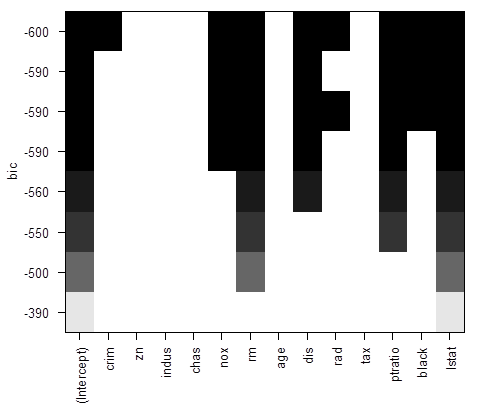
# There is a nice way to visualize results, ranking models by the
chosen “scale”. Black color means the variable is included into the model,
white means it is excluded.
>
plot(reg)
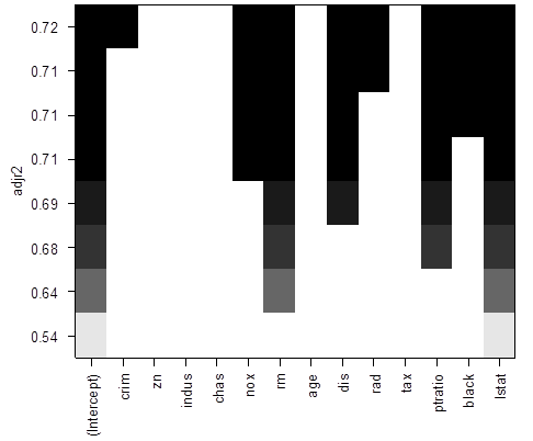
>
plot(reg, scale = "adjr2" )
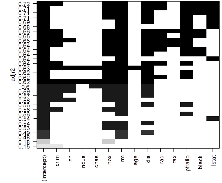
# To see more models, use option “nbest”, which is the number of models of each size p to be
compared.
> reg = regsubsets(
medv ~ ., data=Boston, method = "backward",
nbest=4 )
> plot(reg, scale = "adjr2" )
# We can also choose the best model by means of a stepwise procedure,
starting with one model and ending with another.
> null = lm( medv ~ 1, data=Boston )
> full = lm( medv ~ ., data=Boston )
> step( null, scope=list(lower=null, upper=full),
direction="forward" )
Start: AIC=2246.51
medv ~ 1
Df Sum of
Sq RSS AIC
+ lstat 1
23243.9 19472 1851.0 # Compare contributions of
+ rm 1
20654.4 22062 1914.2 # remaining independent variables
+ ptratio 1
11014.3 31702 2097.6
+ indus 1
9995.2 32721 2113.6
+ tax 1
9377.3 33339 2123.1
+ nox 1
7800.1 34916 2146.5
+ crim 1
6440.8 36276 2165.8
+ rad 1
6221.1 36495 2168.9
+ age 1
6069.8 36647 2171.0
+ zn 1
5549.7 37167 2178.1
+ black 1
4749.9 37966 2188.9
+ dis 1 2668.2 40048 2215.9
+ chas 1
1312.1 41404 2232.7
<none> 42716 2246.5
Step: AIC=1851.01
medv ~ lstat
Df Sum of
Sq RSS AIC
+ rm 1
4033.1 15439 1735.6
+ ptratio 1
2670.1 16802 1778.4
+ chas 1
786.3 18686 1832.2
+ dis 1
772.4 18700 1832.5
+ age 1
304.3 19168 1845.0
+ tax 1
274.4 19198 1845.8
+ black 1
198.3 19274 1847.8
+ zn 1
160.3 19312 1848.8
+ crim 1
146.9 19325 1849.2
+ indus 1
98.7 19374 1850.4
<none> 19472 1851.0
+ rad 1
25.1 19447 1852.4
+ nox 1
4.8 19468 1852.9
... < truncated > ...
Step: AIC=1585.76
medv ~ lstat
+ rm + ptratio + dis + nox
+ chas + black + zn +
crim + rad + tax
Df Sum of
Sq RSS AIC
<none> 11081 1585.8
+ indus 1
2.51754 11079 1587.7
+ age 1
0.06271 11081 1587.8
Call:
lm(formula = medv ~ lstat + rm + ptratio + dis + nox + chas +
black + zn + crim + rad + tax, data = Boston)
Coefficients:
(Intercept) lstat rm ptratio dis nox
36.341145
-0.522553 3.801579 -0.946525
-1.492711 -17.376023
chas black zn crim rad tax
2.718716
0.009291 0.045845 -0.108413 0.299608
-0.011778
#
The final model contains variables lstat,
rm, ptratio, dis, nox, chas, black, zn, crim, rad, and tax.
2. RIDGE REGRESSION
#
Dataset “Boston” has some strong correlations, resulting in multicollinearity.
>
cor(Boston)
#
Apply ridge regression
>
lm.ridge(
medv~., data=Boston, lambda=0.5 )
crim zn indus chas
36.270091954
-0.107524388 0.046092635 0.018815242
2.693518778
nox rm age dis rad
-17.646013524 3.816019080
0.000578687 -1.469191794 0.301928336
tax ptratio black lstat
-0.012134702
-0.950831885 0.009309388 -0.523845421
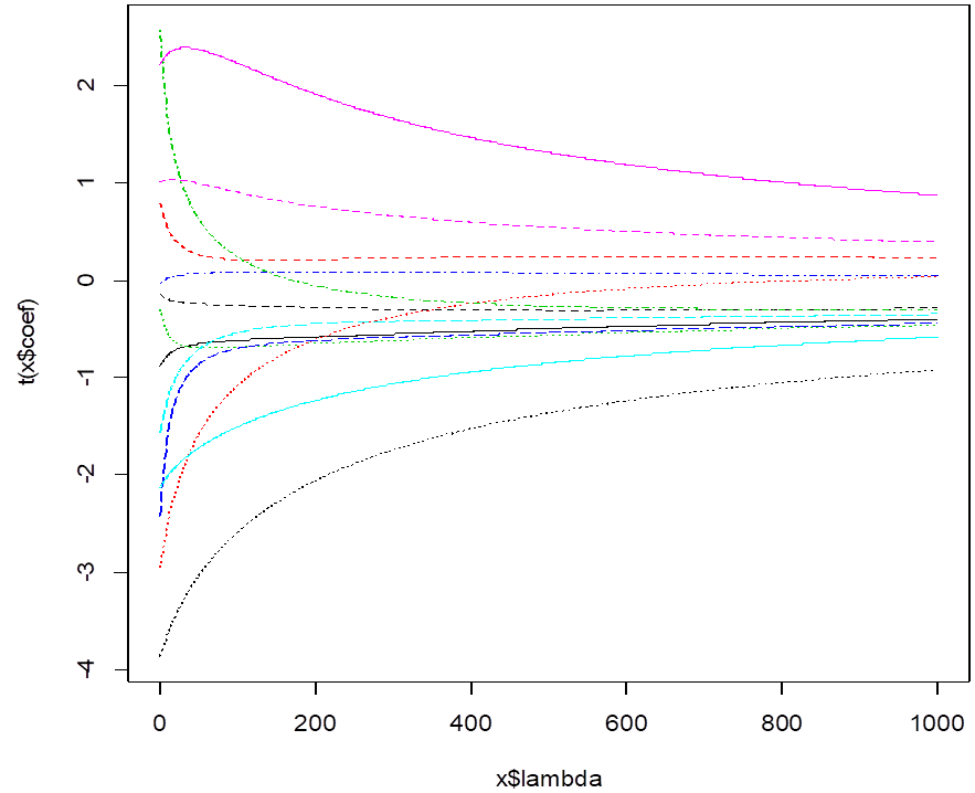
#
We can see how the slopes change with penalty lambda. These are estimated
slopes for different lambda. When lambda=0, we get LSE. Large lambda forces
them toward 0.
>
rr = lm.ridge(medv ~ ., data=train, lambda=seq(0,1000,1) )
>
rr
>
plot(rr)
#
To choose a good lambda, fit ridge regression with various lambda and compare
prediction performance.
> select(rr)
modified HKB
estimator is 4.321483
modified L-W
estimator is 3.682107
smallest value
of GCV at 5
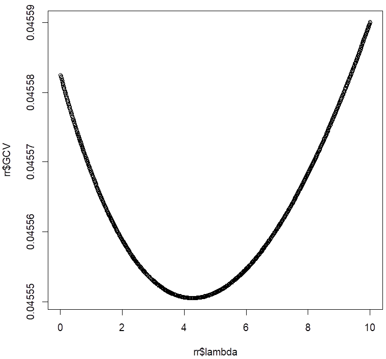
#
So, the best lambda is around 5. We’ll look closer at that range.
> rr = lm.ridge( medv~., data=Boston, lambda=seq(0,10,0.01) )
> select(rr)
modified HKB
estimator is 4.594163
modified L-W
estimator is 3.961575
smallest value
of GCV at 4.26
> plot(rr$lambda,rr$GCV)